Spatial data and the tidyverse

Spatial data and the tidyverse🌐
 new tools for geocomputation with RRobin Lovelace and Jakub Nowosad2017-09-051 / 23

This mini-workshop will introduce you to recent developments that enable work with spatial data 'in the tidyverse'. By this we mean handling spatial datasets using functions (such as %>% and filter()) and concepts (such as type stability) from R packages that are part of the metapackage tidyverse, which can now be installed from CRAN with the following command:

install.packages("tidyverse")

This functionality is possible thanks to sf, a recent package (first release in 2016) that implements the open standard data model simple features. Get sf with:

install.packages("sf")

The workshop will briefly introduce both packages (which should be installed on your computer before attending) before demonstrating how they can work in harmony using a dataset from the spData package, which can be installed with:

install.packages("spData")

The workshop is based on our work on the forthcoming book Geocomputation with R - please take a look at the book and its source code prior to the workshop here: github.com/Robinlovelace/geocompr.

2 / 23

ContextSoftware for 'data science' is evolving
In R, packages ggplot2 and dplyr have become immensely popular and now they are a part of the tidyverse
These packages use the 'tidy data' principles for consistency and speed of processing (from vignette("tidy-data")):

Each variable forms a column.
Each observation forms a row.
Each type of observational unit forms a table

Historically spatial R packages have not been compatible with the tidyverse
3 / 23

4 / 23

Enter sf

sf is a recently developed package for spatial (vector) data
Combines the functionality of three previous packages: sp, rgeos and rgdal
Has many advantages, including:
- Faster data I/O
- More geometry types supported
- Compatibility with the tidyverse

That's the topic of this workshop

5 / 23

Geocomputation with RA book we are working on for CRC Press (to be published in 2018)
Chapters 3 and 4 of this book form the basis of the worked examples presented here
6 / 23

Prerequisites

Install the required packages. You need a recent version of the GDAL, GEOS, Proj.4, and UDUNITS libraries installed for this to work on Mac and Linux. More information on that at https://github.com/r-spatial/sf#installling.

devtools::install_github("robinlovelace/geocompr")

Load the ones we need:

library(spData)
library(dplyr)
library(sf)

Check it's all working, e.g. with this command:

world %>%
  plot()

7 / 23

Reading and writing spatial data

library(sf)
library(spData)
vector_filepath = system.file("shapes/world.gpkg", package = "spData")
vector_filepath

## [1] "/home/robin/R/x86_64-pc-linux-gnu-library/3.4/spData/shapes/world.gpkg"

world = st_read(vector_filepath)

## Reading layer `wrld.gpkg' from data source `/home/robin/R/x86_64-pc-linux-gnu-library/3.4/spData/shapes/world.gpkg' using driver `GPKG'
## Simple feature collection with 177 features and 10 fields
## geometry type:  MULTIPOLYGON
## dimension:      XY
## bbox:           xmin: -180 ymin: -90 xmax: 180 ymax: 83.64513
## epsg (SRID):    4326
## proj4string:    +proj=longlat +datum=WGS84 +no_defs

Counterpart to st_read() is the st_write function, e.g. st_write(world, 'data/new_world.gpkg'). A full list of supported formats could be found using sf::st_drivers().

8 / 23

Structure of the sf objects

world

## Simple feature collection with 177 features and 10 fields
## geometry type:  MULTIPOLYGON
## dimension:      XY
## bbox:           xmin: -180 ymin: -90 xmax: 180 ymax: 83.64513
## epsg (SRID):    4326
## proj4string:    +proj=longlat +datum=WGS84 +no_defs
## First 3 features:
##   iso_a2   name_long continent region_un       subregion              type
## 1     AF Afghanistan      Asia      Asia   Southern Asia Sovereign country
## 2     AO      Angola    Africa    Africa   Middle Africa Sovereign country
## 3     AL     Albania    Europe    Europe Southern Europe Sovereign country
##    area_km2      pop  lifeExp gdpPercap                           geom
## 1  652270.1 31627506 60.37446  1844.022 MULTIPOLYGON (((61.21081709...
## 2 1245463.7 24227524 52.26688  6955.960 MULTIPOLYGON (((16.32652835...
## 3   29694.8  2893654 77.83046 10698.525 MULTIPOLYGON (((20.59024743...

class(world)

## [1] "sf"         "data.frame"

9 / 23

Structure of the sf objects

world$name_long

## [1] Afghanistan Angola      Albania    
## 177 Levels: Afghanistan Albania Algeria Angola Antarctica ... Zimbabwe

world$geom

## Geometry set for 177 features 
## geometry type:  MULTIPOLYGON
## dimension:      XY
## bbox:           xmin: -180 ymin: -90 xmax: 180 ymax: 83.64513
## epsg (SRID):    4326
## proj4string:    +proj=longlat +datum=WGS84 +no_defs
## First 3 geometries:

## MULTIPOLYGON (((61.2108170917257 35.65007233330...

## MULTIPOLYGON (((16.326528354567 -5.877470391466...

## MULTIPOLYGON (((20.5902474301049 41.85540416113...

10 / 23

sf vs sp

The sp package is a predecessor of the sf package
Together with the rgdal and rgeos package, it creates a powerful tool to works with spatial data
Many spatial R packages still depends on the sp package, therefore it is important to know how to convert sp to and from sf objects

library(sp)
world_sp = as(world, "Spatial")
world_sf = st_as_sf(world_sp)

The structures in the sp packages are more complicated - str(world_sf) vs str(world_sp)
Moreover, many of the sp functions are not "pipeable" (it's hard to combine them with the tidyverse)

world_sp %>% 
  filter(name_long == "England")

Error in UseMethod("filter_") : no applicable method for 'filter_' applied to an object of class "c('SpatialPolygonsDataFrame', 'SpatialPolygons', 'Spatial')"

11 / 23

Non-spatial operations on the sf objects

world %>% 
  left_join(worldbank_df, by = "iso_a2") %>%
  select(name_long, pop, pop_growth, area_km2) %>%
  arrange(area_km2) %>% 
  mutate(pop_density = pop/area_km2) %>%
  rename(population = pop)

## Simple feature collection with 177 features and 5 fields
## geometry type:  MULTIPOLYGON
## dimension:      XY
## bbox:           xmin: -180 ymin: -90 xmax: 180 ymax: 83.64513
## epsg (SRID):    4326
## proj4string:    +proj=longlat +datum=WGS84 +no_defs
## First 20 features:
##                              name_long population  pop_growth  area_km2
## 1                           Luxembourg     556319  2.35697870  2416.870
## 2                      Northern Cyprus         NA  2.36947994  3786.365
## 3                            Palestine    4294682  2.95799495  5037.104
## 4                               Cyprus    1153658  1.04614274  6207.006
## 5                              Vanuatu     258883  2.23347721  7490.040
## 6                  Trinidad and Tobago    1354483  0.46197935  7737.810
## 7                          Puerto Rico    3534888 -1.63278794  9224.663
## 8                              Lebanon    5612096  5.96751825 10099.003
## 9                    Brunei Darussalam     417394  1.42240299 10700.334
## 10                              Kosovo         NA  2.36947994 11230.333
## 11                               Qatar    2172065  3.31278379 11327.855
## 12 French Southern and Antarctic Lands         NA          NA 11602.572
## 13                             Jamaica    2720554  0.36303364 12460.587
## 14                          Montenegro     621810  0.09702201 13443.720
## 15                          The Gambia    1928201  3.23199269 14031.284
## 16                         Timor-Leste    1212107  2.45302951 14714.931
## 17                             Bahamas     383054  1.37024992 15584.791
## 18                    Falkland Islands         NA          NA 16363.799
## 19                              Kuwait    3753121  4.34085090 16652.120
## 20                           Swaziland    1269112  1.46612234 18118.634
##    pop_density                           geom
## 1    230.18155 MULTIPOLYGON (((6.043073357...
## 2           NA MULTIPOLYGON (((32.73178022...
## 3    852.60939 MULTIPOLYGON (((35.54566531...
## 4    185.86384 MULTIPOLYGON (((33.97361657...
## 5     34.56363 MULTIPOLYGON (((167.8448767...
## 6    175.04734 MULTIPOLYGON (((-61.68 10.7...
## 7    383.19968 MULTIPOLYGON (((-66.2824344...
## 8    555.70792 MULTIPOLYGON (((35.82110070...
## 9     39.00757 MULTIPOLYGON (((114.2040165...
## 10          NA MULTIPOLYGON (((20.76216 42...
## 11   191.74549 MULTIPOLYGON (((50.81010827...
## 12          NA MULTIPOLYGON (((68.935 -48....
## 13   218.33273 MULTIPOLYGON (((-77.5696007...
## 14    46.25282 MULTIPOLYGON (((19.80161339...
## 15   137.42156 MULTIPOLYGON (((-16.8415246...
## 16    82.37259 MULTIPOLYGON (((124.9686824...
## 17    24.57871 MULTIPOLYGON (((-77.53466 2...
## 18          NA MULTIPOLYGON (((-61.2 -51.8...
## 19   225.38398 MULTIPOLYGON (((47.97451907...
## 20    70.04457 MULTIPOLYGON (((32.07166548...

12 / 23

Non-spatial operations

world_cont = world %>% 
        group_by(continent) %>% 
        summarize(pop_sum = sum(pop, na.rm = TRUE))

## Simple feature collection with 8 features and 2 fields
## geometry type:  GEOMETRY
## dimension:      XY
## bbox:           xmin: -180 ymin: -90 xmax: 180 ymax: 83.64513
## epsg (SRID):    4326
## proj4string:    +proj=longlat +datum=WGS84 +no_defs
## # A tibble: 8 x 3
##   continent    pop_sum              geom
##      <fctr>      <dbl>  <simple_feature>
## 1    Africa 1147005839 <MULTIPOLYGON...>
## # ... with 7 more rows

The st_set_geometry function can be used to remove the geometry column:

world_df =st_set_geometry(world_cont, NULL)
class(world_df)

## [1] "tbl_df"     "tbl"        "data.frame"

13 / 23

Spatial operations

It's a big topic which includes:

Spatial subsetting
Spatial joining/aggregation
Topological relations
Distances
Spatial geometry modification
Raster operations (map algebra)

See Chapter 4 of Geocomputation with R

14 / 23

Spatial subsetting

lnd_buff = lnd[1, ] %>% 
  st_transform(crs = 27700) %>%  # uk CRS
  st_buffer(500000) %>%
  st_transform(crs = 4326)
near_lnd = world[lnd_buff, ]
plot(near_lnd$geom)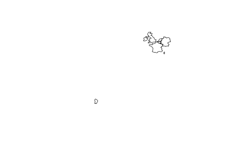

What is going with the country miles away?

15 / 23

Multi-objects

Some objects have multiple geometries:

st_geometry_type(near_lnd)

## [1] MULTIPOLYGON MULTIPOLYGON MULTIPOLYGON MULTIPOLYGON MULTIPOLYGON
## [6] MULTIPOLYGON MULTIPOLYGON
## 18 Levels: GEOMETRY POINT LINESTRING POLYGON ... TRIANGLE

Which have more than 1?

data.frame(near_lnd$name_long,
           sapply(near_lnd$geom, length))

##   near_lnd.name_long sapply.near_lnd.geom..length.
## 1            Belgium                             1
## 2            Germany                             1
## 3             France                             3
## 4     United Kingdom                             2
## 5            Ireland                             1
## 6         Luxembourg                             1
## 7        Netherlands                             1

16 / 23

Subsetting contiguous polygons

near_lnd_new = world %>% 
  st_cast(to = "POLYGON") %>% 
  filter(st_intersects(., lnd_buff, sparse = FALSE))
plot(near_lnd_new$geometry)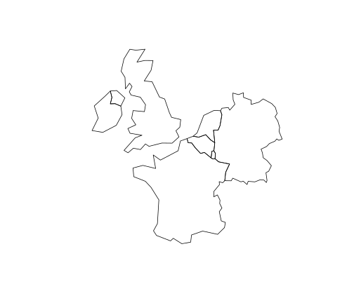

17 / 23

CRS

na_2163 = world %>%
  filter(continent == "North America") %>% 
  st_transform(2163) #US National Atlas Equal Area
st_crs(na_2163)

## $epsg
## [1] 2163
## 
## $proj4string
## [1] "+proj=laea +lat_0=45 +lon_0=-100 +x_0=0 +y_0=0 +a=6370997 +b=6370997 +units=m +no_defs"
## 
## attr(,"class")
## [1] "crs"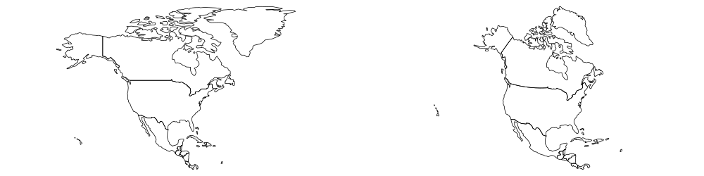

18 / 23

Basic maps

Basic maps of sf objects can be quickly created using the plot() function:

plot(wrld[0])

plot(wrld["pop"])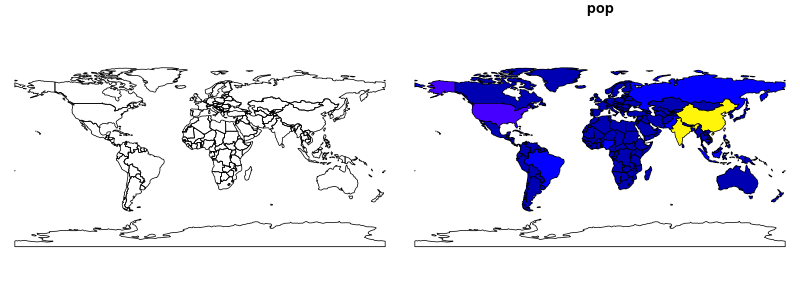

19 / 23

tmap

https://cran.r-project.org/web/packages/tmap/vignettes/tmap-nutshell.html

library(tmap)
tmap_mode("plot") #check the "view"
tm_shape(world, projection="wintri") +
        tm_polygons("lifeExp", title=c("Life expactancy"),
          style="pretty", palette="RdYlGn", auto.palette.mapping=FALSE) +
        tm_style_grey()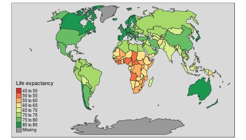

20 / 23

leaflet

library(leaflet)
leaflet(world) %>%
        addTiles() %>%
        addPolygons(color = "#444444", weight = 1, fillOpacity = 0.5,
                    fillColor = ~colorQuantile("YlOrRd", lifeExp)(lifeExp),
                    popup = paste(round(world$lifeExp, 2)))

21 / 23

Raster data in the tidyverse

Raster data is not yet closely connected to the tidyverse, however:

Some functions from the raster package works well in pipes
You can convert vector data to the Spatial* form using as(my_vector, "Spatial")before working on raster-vector interactions
There are some initial efforts to bring raster data closer to the tidyverse, such as tabularaster, sfraster, or fasterize
The development of the stars, package focused on multidimensional, large datasets should start soon. It will allow pipe-based workflows

22 / 23

Geocomputation with R

The online version of the book is at http://robinlovelace.net/geocompr/ and its source code at https://github.com/robinlovelace/geocompr.

We encourage contributions on any part of the book, including:

Improvements to the text, e.g. clarifying unclear sentences, fixing typos (see guidance from Yihui Xie)
Changes to the code, e.g. to do things in a more efficient way
Suggestions on content (see the project's issue tracker and the work-in-progress folder for chapters in the pipeline)

Please see our_style.md for the book's style.

23 / 23

Help

Keyboard shortcuts

↑, ←, Pg Up, k

Go to previous slide

↓, →, Pg Dn, Space, j

Go to next slide

Home

Go to first slide

End

Go to last slide

Number + Return

Go to specific slide

b / m / f

Toggle blackout / mirrored / fullscreen mode

Clone slideshow

Toggle presenter mode

Restart the presentation timer

?, h

Toggle this help

Spatial data and the tidyverse

🌐 new tools for geocomputation with R

Robin Lovelace and Jakub Nowosad

2017-09-05

Context

Enter sf

Geocomputation with R

Prerequisites

Reading and writing spatial data

Structure of the sf objects

Structure of the sf objects

sf vs sp

Non-spatial operations on the sf objects

Non-spatial operations

Spatial operations

Spatial subsetting

Multi-objects

Subsetting contiguous polygons

CRS

Basic maps

tmap

leaflet

Raster data in the tidyverse

Geocomputation with R

Help

🌐
new tools for geocomputation with R