R for Spatial Analysis: futureproof foundations
🌐
from statistical language to GIS
Robin Lovelace
2017-10-10
Introduction
- From the course's home at github.com/Robinlovelace/Creating-maps-in-R and the CDRC website:
This one day course will get you up-to-speed with using R and RStudio for daily working with spatial data. You will learn about R's powerful geospatial data processing, analysis and visualisation capabilities. It is practical and hands-on: you'll learn by doing. It assumes you already use R and want to extend your knowledge for spatial data applications. It will cover the recently developed sf package, which is compatible with the tidyverse, representing the cutting-edge of spatial data applications. It will provide a solid foundation (including spatial aggregation, joining, CRSs, visualisation) on which advanced analysis analysis workflows can be built.
install.packages("tidyverse")Learning outcomes
By the end of the course participants will:
- Understand R's spatial ecosystem and which packages are 'future proof'
- Know how to optimize RStudio for productive working with spatial data (you should already be proficient with RStudio)
- Be able to read and write a variety of spatial data formats
- Be proficient at common spatial operations including subsetting, cropping, aggregation and transformation
- Be a confident map maker using the powerful tmap package
- Know where to look for learning more advanced methods
Prerequisites
In preparation for the course you should:
- Ensure that you have the latest versions of R and RStudio installed on your laptop: https://www.rstudio.com/products/rstudio/download/
- Brush up on your R skills if you're not an R user, e.g. with:
- This excellent tutorial that you can work through to get used to the interface: https://www.datacamp.com/courses/free-introduction-to-r
- A more detailed account by Gillespie and Lovelace (2017): https://csgillespie.github.io/efficientR/set-up.html#rstudio
- Take a look at how GitHub works - we'll be using it for sharing course materials and sharing links and examples during the course, e.g. by reading this page (and following the tutorial if really keen): https://guides.github.com/activities/hello-world/
Test your set-up
This should work:
library(sf)library(raster)library(spData)install.packages("sf")install.packages("spData")Course materials
The course will be based on Chapter 4 of Geocomputation with R of the forthcoming book Geocomputation with R plus some additional materials:
- An introduction to geographic data in R
- Chapter 2 of Geocomputation with R
- Geographic data I/O
- Chapter 5 of Geocomputation with R
- Introduction to visualising spatial data with R
- Creating-maps-in-R GitHub tutorial
- Point pattern analysis and rasterization
- Point Pattern analysis and spatial interpolation with R from the previous tutorial
Course agenda
Refreshments & set-up: (09:00 - 09:30)
- R's spatial ecosystem: (09:30 - 09:40)
- See section 1.4 of Geocomputation with R
- R and RStudio for spatial data (09:40 - 09:50)
- An introduction to simple features (09:50 - 10:00)
- Working with attribute data (10:00 - 10:45)
- Section 3.2 of handouts
Coffee break: (10:45 - 11:00)
- Raster data classes and functions (11:00 - 11:15)
- Online tutorial: 2.2 of Geocomputation with R
- Raster attribute data (11:15 - 12:00)
- Section 3.3 of handouts
- Free working (12:00 - 12:30)
- Challenge: working-through and complete the exercises in Chapter 3
- Bonus: ask a question and help explain something
- Advanced: look into GitHub and data science
LUNCH and looking at your data (12:30 - 13:30)
Worked example: car fleet analysis with Craig Morton (13:30 - 14:15)
Spatial data operations (14:15 - 15:00)
- Practical based on the second handout
- Spatial subsetting, section 4.2.1
- Topological relations
- Spatial joining and aggregation
Coffee break: 15:00 - 15:15
- Geographic data I/O: (15:15 - 15:30)
- Taught lecture
- Test based on your own data
Spatial operations on raster data (15:30 - 15:45)
- Practical - work through section 4.3
Consolidating knowledge (15:45 - 16:15)
- Completing the printed hand-out OR
- Point pattern analysis, interpolation and rasterization tutorial
- Working on your own data
Wrap-up and next steps (16:15 - 16:30)
R's spatial ecosystem

The popularity of spatial packages in R. The y-axis shows the average number of downloads, within a 30-day rolling window, of R's top 5 spatial packages, defined as those with the highest number of downloads last month.
Before spatial packages...
- Coordinates were treated as just another variable
- Issues with visualisation, spatial relations and consistency
- Major issues with Coordinate Reference Systems (CRSs)
library(spData) # see data(package = "spData") and ?afcon for more infoplot(afcon$x, afcon$y)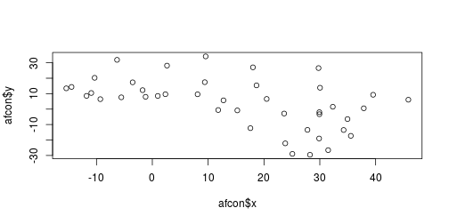
sp
- Released in 2005 (Pebesma and Bivand 2005)
- Raster and vector data (but mostly raster) supported
- We won't be using it but it is useful to know about ()
library(sp)data(meuse)coords = SpatialPoints(meuse[c("x", "y")])meuse = SpatialPointsDataFrame(coords, meuse)str(meuse)## Formal class 'SpatialPointsDataFrame' [package "sp"] with 5 slots## ..@ data :'data.frame': 155 obs. of 14 variables:## .. ..$ x : num [1:155] 181072 181025 181165 181298 181307 ...## .. ..$ y : num [1:155] 333611 333558 333537 333484 333330 ...## .. ..$ cadmium: num [1:155] 11.7 8.6 6.5 2.6 2.8 3 3.2 2.8 2.4 1.6 ...## .. ..$ copper : num [1:155] 85 81 68 81 48 61 31 29 37 24 ...## .. ..$ lead : num [1:155] 299 277 199 116 117 137 132 150 133 80 ...## .. ..$ zinc : num [1:155] 1022 1141 640 257 269 ...## .. ..$ elev : num [1:155] 7.91 6.98 7.8 7.66 7.48 ...## .. ..$ dist : num [1:155] 0.00136 0.01222 0.10303 0.19009 0.27709 ...## .. ..$ om : num [1:155] 13.6 14 13 8 8.7 7.8 9.2 9.5 10.6 6.3 ...## .. ..$ ffreq : Factor w/ 3 levels "1","2","3": 1 1 1 1 1 1 1 1 1 1 ...## .. ..$ soil : Factor w/ 3 levels "1","2","3": 1 1 1 2 2 2 2 1 1 2 ...## .. ..$ lime : Factor w/ 2 levels "0","1": 2 2 2 1 1 1 1 1 1 1 ...## .. ..$ landuse: Factor w/ 15 levels "Aa","Ab","Ag",..: 4 4 4 11 4 11 4 2 2 15 ...## .. ..$ dist.m : num [1:155] 50 30 150 270 380 470 240 120 240 420 ...## ..@ coords.nrs : num(0) ## ..@ coords : num [1:155, 1:2] 181072 181025 181165 181298 181307 ...## .. ..- attr(*, "dimnames")=List of 2## .. .. ..$ : chr [1:155] "1" "2" "3" "4" ...## .. .. ..$ : chr [1:2] "x" "y"## ..@ bbox : num [1:2, 1:2] 178605 329714 181390 333611## .. ..- attr(*, "dimnames")=List of 2## .. .. ..$ : chr [1:2] "x" "y"## .. .. ..$ : chr [1:2] "min" "max"## ..@ proj4string:Formal class 'CRS' [package "sp"] with 1 slot## .. .. ..@ projargs: chr NAsp visuals
12 year-old code still works (Pebesma and Bivand 2005)
plot(meuse, pch=1, cex = .05*sqrt(meuse$zinc))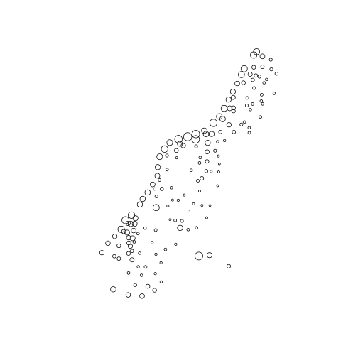
Packages building on sp
sp has many reverse dependencies:
sp_revdeps = devtools::revdep("sp", dependencies = "Depends")head(sp_revdeps)## [1] "adehabitat" "adehabitatHR" "adehabitatHS" "adehabitatLT"## [5] "adehabitatMA" "automap"length(sp_revdeps)## [1] 135sp_revimps = devtools::revdep("sp", dependencies = "Imports")length(sp_revimps)## [1] 256Where to find out about packages?
Online (dur) but with guidance, e.g. from:
- The Spatial Taskview: https://cran.r-project.org/web/views/Spatial.html
- Section 4.4. of Efficient R Programming
A few of note:
- adehabitat for ecological modelling
- geosphere for operations on a spherical surface
- spdep for modelling spatial data
- rgdal for reading/writing data
The 5 most downloaded packages that depend on sp

sf
- Released in November 2016
- Aims to supersede sp, rgdal and rgeos with unified interface
- Treats spatial vector data as regular data frames
- The basis of much of this tutorial and Geocomputation with R
- Compatible with the tidyverse (Wickham and Grolemund 2016)
library(sf)## Linking to GEOS 3.5.1, GDAL 2.2.1, proj.4 4.9.2, lwgeom 2.3.3 r15473world_tbl = dplyr::as_data_frame(world)world_tbl## # A tibble: 177 x 11## iso_a2 name_long continent## <chr> <chr> <chr>## 1 AF Afghanistan Asia## 2 AO Angola Africa## 3 AL Albania Europe## 4 AE United Arab Emirates Asia## 5 AR Argentina South America## 6 AM Armenia Asia## 7 AQ Antarctica Antarctica## 8 TF French Southern and Antarctic Lands Seven seas (open ocean)## 9 AU Australia Oceania## 10 AT Austria Europe## # ... with 167 more rows, and 8 more variables: region_un <chr>,## # subregion <chr>, type <chr>, area_km2 <dbl>, pop <dbl>, lifeExp <dbl>,## # gdpPercap <dbl>, geom <simple_feature>raster
- A very large package first released in 2010
- Provides support for raster classes, and user friendly functions for vector data
- Very powerful
library(raster)r = raster(nrows = 3, ncols = 3)values(r) = 1:9plot(r)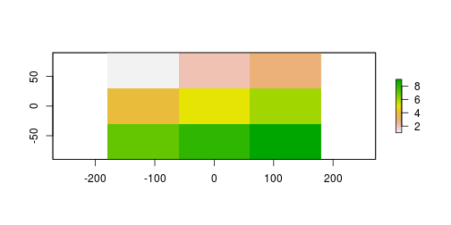
Visualisation packages
- ggplot2 support for sf
- leaflet for low-level control of interactive maps
- mapview for GIS-like feel
- tmap powerful, flexible, user-friendly, general-purpose map-making
References
Grolemund, G., Wickham, H., 2016. R for Data Science, 1 edition. ed. O’Reilly Media.
Lovelace, R., Nowosad, J., Meunchow, J., 2018. Geocomputation with R. CRC Press.
Pebesma, E.J., Bivand, R.S., 2005. Classes and methods for spatial data in R. R news 5, 9–13.
Links and example code from the course in Leeds: https://github.com/Robinlovelace/Creating-maps-in-R/blob/master/courses/leeds-2017-10.Rmd
Plug: GIS for Transport Applications: https://www.eventbrite.co.uk/e/gis-for-transport-applications-tickets-38491819067